In this post, we’ll take a database of quotations from Hugging Face, convert it to a NetworkX object using Semnet, and examine how we can use graph structures to enrich and manipulate a text corpus.

Building the network

First we load in the data and embed our documents. Semnet operates on a “bring your own embeddings” model, allowing for any numpy array to be used to build your network. Here I use sentence-transformers.

import datasets
import sentence_transformers

# Load data
dataset = datasets.load_dataset("m-ric/english_historical_quotes")

# Get quotes
labels = [item["quote"] for item in dataset["train"]]

# Embed texts
model_str = "BAAI/bge-base-en-v1.5"
embedding_model = sentence_transformers.SentenceTransformer(model_str)
embeddings = embedding_model.encode(labels, show_progress_bar=True)

Checking the length of the data, we see we have just over 24 thousand records.

print(len(embeddings))
>> 24022

We can then easily convert the labels and embeddings to a network using Semnet. The below runs in just under eight seconds on my four-year-old gaming laptop, much faster than when doing the embedding.

from semnet import SemanticNetwork

# Fit the network, passing in custom data
sem = SemanticNetwork()

# We can pass in arbitrary node data as a dictionary
node_data = {}
for n, item in enumerate(dataset):
    node_data[n] = {"author": item["author"], "foo": "bar"}

G = sem.fit_transform(
    embeddings=embeddings,
    labels=labels,  # labels can be optionally passed during fitting
    thresh=0.25,
    top_k=20,
    node_data=node_data,
)

Exploring the network

We now have a networkx graph we can manipulate as we please.

print(f"G is of type: {type(G)}")
n_nodes, n_edges = G.number_of_nodes(), G.number_of_edges()
print(f"G has {n_nodes} nodes and {n_edges} edges.")

G is of type: <class 'networkx.classes.graph.Graph'>
G has 24022 nodes and 40559 edges

We can take a look at the nodes:

import random
random.seed(123)

# Take a random sample
print("Sample nodes:")
sample = random.sample(list(G.nodes(data=True)), 5)

# Print out the author and a cropped quote
for idx, node in sample:
   print(f'{node["author"]}: "{node["label"][:30]}..."')

Sample nodes:
Archimedes: "Give me a lever long enough an..."
Graham Greene: "If you have abandoned one fait..."
Betty White: "My mother and dad were big ani..."
Joyce Carol "Oates: I could never take the idea of..."
Gore Vidal: "We must declare ourselves, bec..."

And the edges:

print("Sample edges:")

# Take a random sample
random.seed(123)
sample = random.sample(list(G.edges(data=True)), 5)

# Order by weight
for u, v, edge in sorted(sample, key=lambda x: x[2]["weight"], reverse=True):
    quote_u = G.nodes[u]["label"][:30]
    quote_v = G.nodes[v]["label"][:30]
    print(f'"{quote_u}" {edge["weight"]:.2f} "{quote_v}"')

Sample edges:
"We extend our hand towards pea" 0.32 "Our object should be peace wit"
"Death is really a great blessi" 0.30 "Life is a great sunrise. I do "
"Love is the river of life in t" 0.26 "People think love is an emotio"
"No amount of skillful inventio" 0.25 "Anyone who lives within his me"
"I have a fine sense of the rid" 0.25 "I don't think humor is forced "

Connectivity

Unless we’ve set our parameters for a very dense graph during construction (i.e., with a low thresh and a high top_k), we are likely to see a lot of unconnected components, orphan nodes with no relationship to each other.

This is a trade-off during graph construction. We can choose to have a heavily-connected graph with a large memory footprint and tenuous links; or a sparser, leaner graph which models only the strongest relationships at the cost of increasing numbers of orphaned (unconnected) nodes.

import networkx as nx

# Get connected components
components = list(nx.connected_components(G))
print(f"\nThe graph has {len(components)} connected components.")


# Count how many components of each size there are
from collections import Counter
component_sizes = [len(c) for c in components]
component_size_counts = Counter(component_sizes)

for size, count in sorted(component_size_counts.items(), reverse=True):
    print(f"Size {size}: {count} components")

With this graph, we can see around half the graph is one large component with 11,471 nodes, the other half of the graph has no or few neighbours and is unconnected to the main body.

Disconnected nodes are challenging for network analysis, as they lie outside the main graph, and as such are inaccessible to many algorithms.

The graph has 11854 connected components.
Size 11471: 1 components
Size 11: 1 components
Size 10: 1 components
Size 8: 1 components
Size 7: 3 components
Size 6: 3 components
Size 5: 5 components
Size 4: 17 components
Size 3: 76 components
Size 2: 416 components
Size 1: 11330 components

As this is demonstration, I will just drop everything but the largest group.

# Keep track of the old size
old_size = len(G.nodes)

# Use networkx to find the subgraph
subgraphs = list(nx.connected_components(G))
largest_subgraph = max(subgraphs, key=len)

# Reduce the graph down
G = G.subgraph(largest_subgraph).copy()

# Print out reduction
new_size = len(G.nodes)
print(
    f"""Reduced graph from {old_size} to {new_size}.
{old_size - new_size} nodes were removed."""
)

Reduced graph from 24022 to 11471.
12551 nodes were removed.

It’s a lossy approach, dropping over half our data, but this is just a demo so let’s proceed.

If you’d like to find out more about dealing with disconnected components, check out the parameters section on the docs.

Graph algorithms

Now that we’ve cleaned up our graph, we can get on with the good stuff. Consider the following examples as inspiration, but there are hundreds of different graph algorithms exposed by the graph structure to experiment with.

I encourage you to take some time to explore the NetworkX documentation and find what works for your specific use case.

Get a node’s neighbours

NetworkX makes it easy to get a node’s neighbours, allowing us to quickly explore local structure.

# Get a node's neighbours
random.seed(1234)
sample_node = random.choice(list(G.nodes(data=True)))
neighbors = list(G.neighbors(sample_node[0]))

# Print the sample node and its neighbors
print(f"Sample node: {sample_node[1]['label'][:50]}...")
print("Neighbors:")
for neighbor in neighbors:
    print(f"- {G.nodes[neighbor]['label'][:50]}...")

Sample node: Anything in any way beautiful derives its beauty f...
Neighbors:
- If thou desire the love of God and man, be humble,...
- Beauty is but the sensible image of the Infinite. ...
- Beauty, like truth, is relative to the time when o...
- Man's only true happiness is to live in hope of so...
- The thought came to me that all one loves in art b...
- Love of beauty is taste. The creation of beauty is...
- An act of goodness is of itself an act of happines...
- Always think of what is useful and not what is bea...
- Beauty is an ecstasy it is as simple as hunger. Th...

Find the shortest path between two nodes

A fun and interesting way of looking at relationships in a semantic network is to find the shortest path between two nodes. This gives us a sense of how two texts are related via intermediate texts.

random.seed(1)

# Sample two random nodes
node_a, node_b = random.sample(list(G.nodes(data=True)), 2)

# Our weights are similarity scores, so we need to invert them for shortest path
weight_func = lambda u, v, d: 1 - d["weight"]

# Find shortest path
path = nx.shortest_path(G, source=node_a[0], target=node_b[0], weight=weight_func)

# Print the path
print("\nShortest path between two random nodes:\n")
print(f"Source: {node_a[1]['label'][:50]}...")
print(f"Target: {node_b[1]['label'][:50]}...")

for idx in path:
    if idx != node_a[0] and idx != node_b[0]:
        print(f"- {G.nodes[idx]['label'][:50]}...")

Shortest path between two random nodes:

Source: Traveling is seeing it is the implicit that we tra...
Target: Without God, democracy will not and cannot long en...
- To travel is to take a journey into yourself....
- Life isn't about finding yourself. Life is about c...
- The good life is a process, not a state of being. ...
- Life is made up of small pleasures. Happiness is m...
- Happiness is neither without us nor within us. It ...
- God cannot give us a happiness and peace apart fro...

Centrality measures

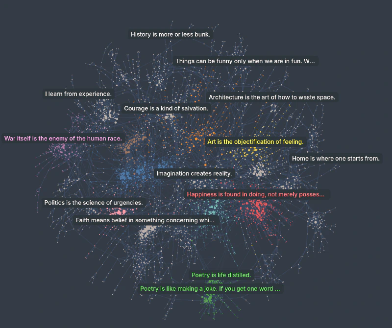
Centrality measures help us identify the most important nodes in a graph. There are several ways to define centrality, but some of the most common include degree centrality, closeness centrality, and betweenness centrality.

Degree centrality represents the number of connections a node has. Closeness centrality measures how close a node is to all other nodes in the graph.

Betweeness centrality is a little more complex, representing the extent to which a node acts as a bridge between other nodes. It can be quite computationally expensive on larger datasets, particularly those with lots of edges.

# Calculate degree centrality
centrality = nx.degree_centrality(G)
nx.set_node_attributes(G, centrality, "degree_centrality")

# Calculate closeness centrality
closeness = nx.closeness_centrality(G)
nx.set_node_attributes(G, closeness, "closeness_centrality")

# Calculate betweenness centrality (can take a while on large graphs)
betweenness = nx.betweenness_centrality(G)
nx.set_node_attributes(G, betweenness, "betweenness_centrality")

This handy chart from Wikipedia gives an intuitive feel for some of the more popular centrality measures.

Exactly how these metrics can be applied will depend on your use case and the dataset.

In the context of quotations, measures of global importance such as pagerank or closeness centrality might help identify influential quotes that connect different themes.

from semnet import to_pandas

nodes, edges = to_pandas(G)

# Sort nodes by closeness centrality
top_pr = nodes.sort_values(by="closeness_centrality", ascending=False)
print("Top 10 Influential Quotes by Closeness Centrality:\n")
for _, row in top_pr.head(10).iterrows():
    print(f'{row["label"][:50]}... [{row["closeness_centrality"]:.6f}]')

Top 10 Influential Quotes by Closeness Centrality:

Human nature is not of itself vicious.... [0.224541]
There are truths which are not for all men, nor fo... [0.221793]
Man is not the creature of circumstances, circumst... [0.219782]
Achieving life is not the equivalent of avoiding d... [0.218539]
Man's nature is not essentially evil. Brute nature... [0.216219]
Men are born to succeed, not to fail.... [0.215326]
Common sense is not so common.... [0.213451]
The good life is a process, not a state of being. ... [0.213173]
However great an evil immorality may be, we must n... [0.212561]
Wise men make more opportunities than they find.... [0.212553]

We could also do the same by author.

author_pr = (
    nodes.groupby("author")["closeness_centrality"]
    .mean()
    .reset_index()
    .sort_values(by="closeness_centrality", ascending=False)
    .head(10)
)

print("Top 10 Influential Authors by Closeness Centrality:\n")
for _, row in author_pr.iterrows():
    print(f'{row["author"][:50]}... [{row["closeness_centrality"]:.6f}]')

Top 10 Influential Authors by Closeness Centrality:

Curt Siodmak... [0.210328]
Amelia Edith Huddleston Barr... [0.210139]
Elizabeth Gaskell... [0.207463]
Conrad Hilton... [0.206443]
Maharishi Mahesh Yogi... [0.206354]
Willy Brandt... [0.206273]
Edmund Waller... [0.205740]
Conor Cruise O'Brien... [0.205721]
Morarji Desai... [0.205688]
Winifred Holtby... [0.202307]

I’m not entirely sure if those are the quotes or authors I’d have picked, but your milage may vary depending on the dataset, the measure of centrality and your research question.

Community detection

Networks can also be used for clustering, or “community detection” in network lingo. Just as we can use something like the excellent BERTopic to identify groups of similar texts using spatial clustering, we can use networkx to perform relationship-based clustering.

Below I briefly demonstrate how we can find Louvain communities, but NetworkX has many different partitioning and community detection algorithms to explore.

communities = nx.community.louvain_communities(G)

for i, community in enumerate(communities):
    for node in community:
        G.nodes[node]["community"] = f"community*{i}"

We can use TF-IDF to label communities.

from sklearn.feature_extraction.text import TfidfVectorizer
import pandas as pd
from semnet import to_pandas

# Get the TF-IDF vectors for the labels
vectorizer = TfidfVectorizer(stop_words="english", max_features=1000)
X = vectorizer.fit_transform(nodes["label"])

# Extract to a dataframe
terms = vectorizer.get_feature_names_out()
tfidf_df = pd.DataFrame(X.toarray(), columns=terms)
tfidf_df["community"] = nodes["community"].values

# Get the top terms
top_terms = {}

# Iterate over community
for community in tfidf_df["community"].unique():

    # Locate the tf-idf matrix at the community
    community_df = tfidf_df[tfidf_df["community"] == community]

    # Get mean tf-idf per term in community
    m_tfidf = community_df.drop(columns=["community"]).mean()

    # Get top 3 terms
    com_terms = m_tfidf.sort_values(ascending=False).head(3).index.tolist()
    top_terms[community] = "_".join(com_terms)

# Create dataframe
nodes, edges = to_pandas(G)

# Map onto nodes dataframe
nodes["top_terms"] = nodes["community"].map(top_terms)

for community, terms in top_terms.items():
    print(f"Top terms for {community}: {terms}")

We can see from the terms that we have communities that appear to have some internal consistency.

Top terms for community_10: humor_funny_sense
Top terms for community_24: success_failure_work
Top terms for community_12: sports_game_like
Top terms for community_29: freedom_government_power
Top terms for community_8: knowledge_education_wisdom
Top terms for community_16: travel_want_life
Top terms for community_23: art_beauty_nature
...
Top terms for community_32: acting_like_imagination

We can also inspect their contents.

# Sample from within top 5 communities
for community in nodes["community_label"].value_counts().head(5).index:
    comm_df = nodes[nodes["community_label"] == community]
    sample_quotes = comm_df.sample(3, random_state=123)
    print(f"\nSample quotes from community '{community}' ({len(comm_df)} items):\n")
    for _, row in sample_quotes.iterrows():
        print(f'- {row["label"][:100]}...')

They hold up pretty well to inspection.

Sample quotes from community 'knowledge_education_wisdom' (1111 items):

- The ultimate goal of the educational system is to shift to the individual the burden of pursing his ...
- A prudent question is one-half of wisdom....
- Any intelligent fool can make things bigger and more complex... It takes a touch of genius - and a l...

Sample quotes from community 'god_faith_religion' (999 items):

- If you don't do your part, don't blame God....
- The investigator should have a robust faith - and yet not believe....
- Uncontrolled, the hunger and thirst after God may become an obstacle, cutting off the soul from what...

Sample quotes from community 'success_failure_best' (892 items):

- Develop success from failures. Discouragement and failure are two of the surest stepping stones to s...
- Success can't be forced....
- There's no such thing as failure - just waiting for success....

Sample quotes from community 'freedom_government_power' (762 items):

- Over grown military establishments are under any form of government inauspicious to liberty, and are...
- To be free in an age like ours, one must be in a position of authority. That in itself would be enou...
- Freedom prospers when religion is vibrant and the rule of law under God is acknowledged....

Sample quotes from community 'happiness_life_happy' (727 items):

- One's philosophy is not best expressed in words it is expressed in the choices one makes... and the ...
- Life is a gift, given in trust - like a child....
- Preoccupation with money is the great test of small natures, but only a small test of great ones....

Exporting

And finally, we can export to pandas for visualisation and downstream tasks.

from semnet import to_pandas

nodes, edges = to_pandas(G)

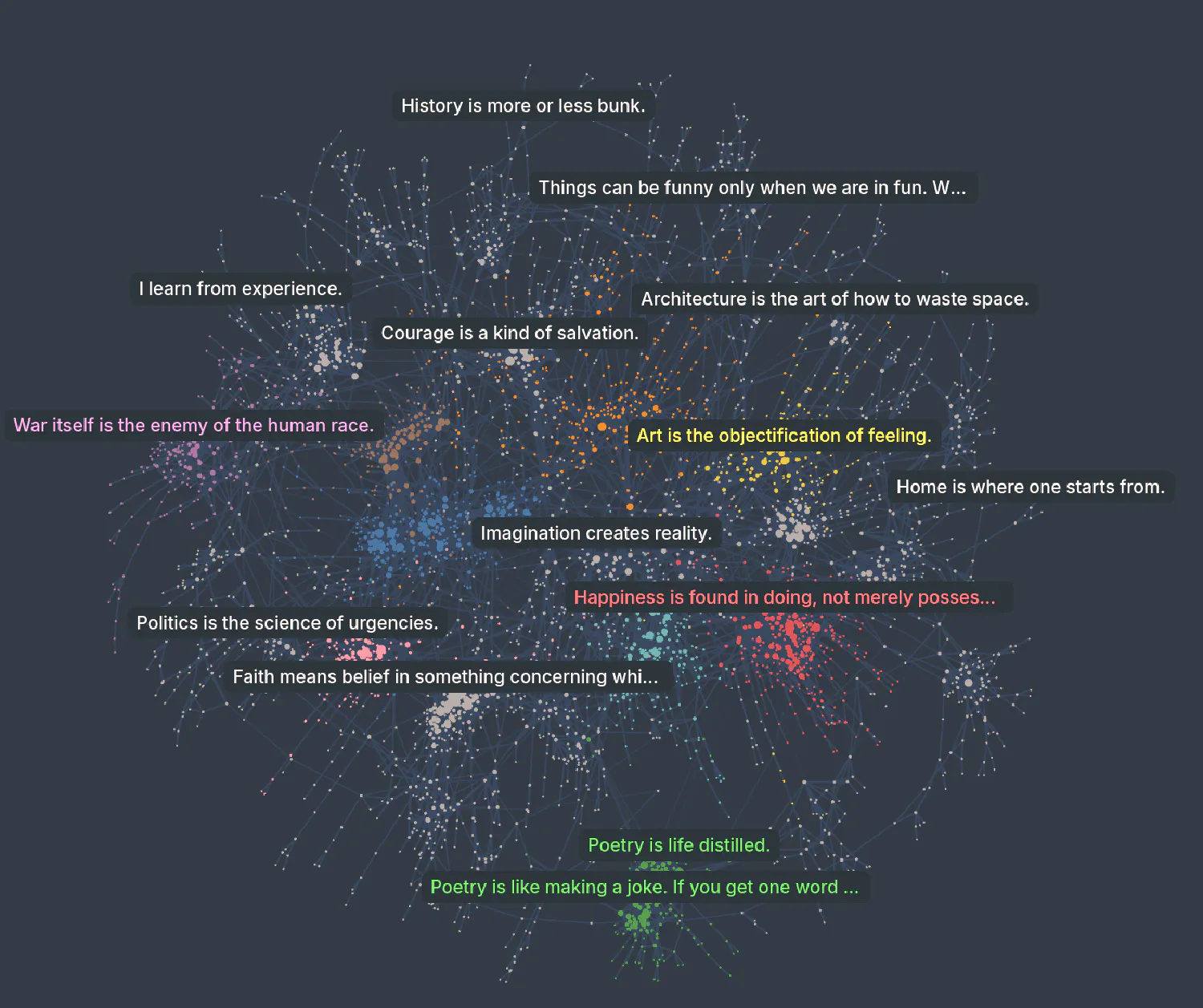
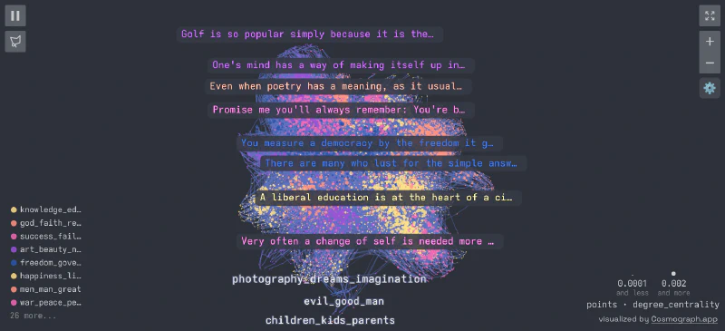
Visualisation

We can visualise in our IDE with the Cosmograph widget.

from cosmograph import Cosmograph

cosmo = Cosmograph(
    points=nodes,
    links=edges,
    point_id_by="node_id",
    point_size_by="degree_centrality",
    link_source_by="source",
    link_target_by="target",
    point_color_by="top_terms",
    point_cluster_by="top_terms",
    point_label_by="label",
    show_cluster_labels=True,
    point_include_columns=["author", "degree_centrality", "betweenness_centrality", "top_terms"],
)
cosmo

Which is pretty cool in itself. That said, the Cosmograph Python widget is in pretty early release, and I find running it in the browser at cosmograph.app to be a smoother experience overall.

We can export our data to a csv for visualisation. Cosmograph expects an id column.

nodes.rename(columns={"node_id": "id"}).to_csv("quotes_nodes_big.csv", index=False)
edges.to_csv("quotes_edges_big.csv", index=False)

We can then head over to the Cosmograph website and visualise. You can check out a pre-made network, built from the data we used in this example here on Cosmograph.

Conclusion

In this post, I’ve demonstrated how to use Semnet to build a semantic network from text embeddings, and given a taste for how NetworkX and graph analysis might be used on an embedded dataset.

Semnet is a flexible tool that can be used with any kind of embedding, not just text. You can build networks from images, audio, even other graphs.

I’d stress again that these examples are simply a starting point. I believe there’s a lot network analysis can bring to NLP and I’d be excited to hear if you find an interesting use for it.

Learn more:

• Check out the repo
• Read the docs